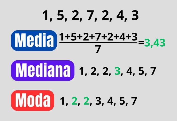
Statistics can seem like a foreign language until you break it down. At the heart of data analysis are three simple tools that tell you where the data set actually lies. We call them measures of central tendency. They answer the question: If you had to pick one number to represent all of this data, what would it be?
These are not just abstract mathematical concepts. They are practical ways to find patterns in chaos. Whether you’re a student staring at an assignment or a parent trying to make sense of your child’s report card, knowing how to calculate the mean, median, and mode makes all the difference.
“Measures of central tendency identify the center of a data set. They show where the most values are clustered.”
Here is a simple breakdown of these three different variables.
Average: mathematical average
The mean is what most people think of when they hear “average.” It is the most commonly used measure, but it is also the most sensitive to outliers.
To find the mean, you follow two simple steps:
1. Add up all the values in the data set.
2. Divide the total by the number of added numbers.
If you have five test results, add them all together and divide by five. The result is the mean. You get an accurate mathematical center, but it can be skewed if one value is significantly higher or lower than the others.
The Median: The Middle Ground
The median is the true middle value of the data set. It’s not the size of the numbers that matters, but their order. This makes it a robust measure when there are outliers that can skew the average.
To calculate the median:
– Arrange your data in ascending order (smallest to largest).
– Find the exact middle number.
If you have an odd number of data points, the median is the single middle value. Usually, when you have an even number, you average the two middle numbers. The median splits the sequence into two equal halves. Half of the data is above this; half is down.
The Mode: The Most Frequent Value
The mode is the simplest concept but can also be the most interesting. It is simply the value that occurs most often in your data set.
A dataset can have:
– One mode (unimodal)
– Two modes (bimodal)
– Multiple modes (multimodal)
– No mode at all (when each value occurs only once)
The mode is particularly useful for categorical data. You can’t calculate the average of your favorite colors, but you can easily find the mode. It tells you what is most common or popular in your group.
Why These Three Matter
Understanding how to calculate the mean, median, and mode isn’t just about passing a test. It is about interpreting of the world.
Imagine looking at house prices in a neighborhood. If one mansion is worth $10 million and nine homes are worth $300,000, the mean price will be dragged up significantly. It might suggest the neighborhood is much more expensive than it actually is for the average buyer. However, the median will remain closer to $300,000, which gives a more realistic picture of typical home costs.
The mean uses every value. The median just uses
Choosing Between Average, Median, and Mode
The choice between mean, median, and mode depends entirely on how your data is distributed. The mean works best when data clusters in the center, offering a accurate picture of the general trend. But if the data skews toward one extreme, the mean gets distorted by outliers.
When values at the extremes differ significantly from the rest, the median or mode often tells a truer story. They highlight what is actually common in your sample or population. Keep in mind that the mode—the most frequent value—can appear anywhere in the dataset, not just in the middle.
Let’s look at a quick example to see how these calculations work. Imagine a fictional ice cream shop tracking monthly sales regardless of flavor:
| Month | Ice Creams Sold |
|---|---|
| January | 41 |
| February | 38 |
| March | 74 |
| April | 98 |
| May | 140 |
| June | 421 |
| July | 785 |
| August | 723 |
| September | 506 |
| October | 140 |
| November | 87 |
| December | 52 |
To find the mean, add all the ice creams sold and divide by the number of months. The result is approximately 259 ice creams per month.
What about the median? First, order the values from smallest to largest:
38 < 41 < 52 < 74 < 87 < 98 < 140 < 140 < 421 < 506 < 723 < 785
Since there is an even number of data points, take the two middle values: 98 and 140. Calculate their average to get the median, which is 119.
Finally, the mode is simply the repeated value. Here, it is 140, as it appears twice while no other number repeats.
How the Mean Is Calculated
The mean is the arithmetic average of a set of numbers. Because it accounts for every single data point, it is highly sensitive to outliers—those extreme values that sit far away from the rest.
Calculating it is straightforward:
- Gather all data points from your sample. No need to sort them first.
- Sum all the data values.
- Divide that total by the count of data points.
Note that this calculation requires numerical data. You cannot calculate a mean for categorical data like colors or names.
Consider a different example: tracking soda consumption among ten people.
| Person | Sodas Consumed |
|---|---|
| A | 5 |
| B | 4 |
| C | 8 |
| D | 5 |
| E | 16 |
| F | 0 |
| G | 10 |
| H | 9 |
| I | 20 |
| J | 1 |
Summing these values gives 78. With 10 people in the sample, dividing 78 by 10 yields a mean of 7.8 sodas per person.
Now, look at how outliers skew this result. Imagine the top ten goal-scorers on a soccer team:
| Player | Goals |
|---|---|
| A | 2 |
| B | 3 |
| C | 4 |
| D | 4 |
| E | 5 |
| F | 6 |
| G | 8 |
| H | 9 |
| I | 12 |
| J | 50 |
The sum is 103. Dividing by 10 players gives a mean of 10.3 goals. It might seem logical to say the average player scores 10.3 goals. But that is misleading. In reality, only two players are above that average. The majority score fewer than 10.
The mean isn’t always the best tool for understanding population behavior. It shines when data is evenly distributed. When skewness exists, you need a different perspective.
Why Median and Mode Matter More in Skewed Data
The median represents the middle point of a dataset. It splits your data in half—50% of values are lower, 50% are higher. Because it relies on position rather than magnitude, it ignores the actual distance between values. This makes it robust against extreme outliers.
In the ice cream example, the median (119) was much closer to the typical monthly sales than the mean (259). The huge summer spikes pulled the mean up, creating a false impression of what a “standard” month looks like. If you run a business, knowing that 119 is a more realistic baseline helps with inventory planning. The mean might lead you to overstock during slower months.
The mode adds another layer of insight. It identifies the most popular outcome. In sales, this is often more actionable than an average. If 140 units are the most common sales figure, that is a pattern worth noting. It tells you what customers actually do most often, not what the mathematical center suggests.
Consider a scenario where you are analyzing customer support ticket resolution times. Most tickets take two days. A few take two weeks due to complex issues. The mean might show 4 days. The median might show 2 days. The mode is definitely 2 days.
Which one is more useful?
If you are setting customer expectations, the median or mode is better. You don’t want to promise 4 days when most people get help in 2. The mean is hiding the reality of your standard service level.
However, the mode has its limits. What if every value is unique? Then there is no mode. Or what if there are multiple modes? A dataset could be bimodal, with two common values. This might indicate two distinct customer groups or product preferences. In such cases, the mode highlights segmentation rather than a single central tendency.
The median is always defined for numerical data, provided you can order it. It is the go-to for income distribution, housing prices, or any dataset where a few extreme values would distort the average.
So, when should you use which?
Use the mean for symmetric distributions with few outliers. Think test scores in a well-balanced class or manufacturing tolerances.
Use the median when data is skewed or has outliers. Think income, house prices, or response times.
Use the mode for categorical data or to find the most frequent occurrence in any dataset. Think favorite colors, preferred payment methods
How to find the median of a data set
The median is the middle value in an ordered list. It is a statistical tool that cuts a data set in half. Unlike the average, it does not allow extreme deviations to distort the result. This makes it reliable for income data or test scores where a crazy high number skews the average.
To find it, you have to follow a strict process. First, collect your numerical data. Sort next. Order matters here. List the numbers from smallest to largest or largest to smallest. The direction does not change the center. After sorting, find the middle.
The method changes depending on whether you have an even or odd number. If the data set contains an odd number of elements, the median is the single value exactly in the middle. If it’s even, you have the middle two numbers. You get the average of these two values. That’s it. Simple logic.
Let’s look at a concrete example. Imagine you are tracking TV sales across seven models.
| Model | Sales |
|---|---|
| A | 104 |
| B | 67 |
| C | 122 |
| D | 176 |
| E | 81 |
| F | 130 |
| G | 75 |
Sort the sales numbers first:
67, 75, 81, 104, 122, 130, 176
There are seven values. The fourth is in the middle. The median is 104. Why? Because there are three numbers below and three above. It sits right in the middle.
Now what happens if you add another TV model? Let’s say Model H, which sold 150 units. The new list looks like this:
67, 75, 81, 104, 122, 130, 150, 176
The count is now even. Eight items. There is no single middle number. You have two: 104 and 122. Take the average of the two.
104 + 122 = 226
226/2 = 113
The new median is 113. It reflects the change in the data distribution.
Identifying the Mode: from numbers to categories
Mode is different. It is the most common value. The size of the numbers doesn’t matter. It’s all about repetition. This makes it unique because it also works with non-numeric data. You can find the mode of eye colors, favorite foods or car brands.
A dataset can have no mode. It can have one. Or it can have many. Terminology changes with frequency.
* Unimodal: One value occurs most often.
* Amodal: No value repeats. Each item is unique.
* Bimodal: Two values share the peak position of the frequency.
* Multimodal: More than two values result in the highest frequency.
Calculate it simply by counting the occurrences. Group the repeated data. Choose the group with the highest number. This is the mode.
Consider surveying ten families and their car ownership.
| Family | Cars |
|---|---|
| A | 1 |
| B | 3 |
| C | 1 |
| D | 2 |
| E | 2 |
| F | 4 |
| G | 2 |
| H | 1 |
| I | 2 |
| J | 3 |
Count the frequencies:
* 4 cars: 1 family
* 3 cars: 2 families
* 1 car: 3 families
* 2 cars: 4 families
Number 2 is the most common. The mode is 2. Most families in this sample own two cars.
The mode shines with categorical data. Look at a study on children’s favorite colors.
| child | Favorite color |
|---|---|
| A | Green |
| B | Red |
| C | Blue |
| D | Green |
| E | White |
| F | Pink |
| G | Purple |
| H | Green |
| I | Blue |
| J | Blue |
Count the colors:
* Green: 3 times
* Blue: 3 times
* Red, White, Pink, Purple: 1 time each
Green and blue share the top spot. This is a bimodal distribution. Both green and blue are the modes. This insight tells you something that the median or mean could never tell you: there is no single “average” preference, only two dominant choices.