Linear programming isn’t just abstract math. It’s the engine behind logistics, supply chains, and resource management. At its core is the simplex method. This standard technique finds the best possible outcome in a system defined by constraints and an objective function.
Think of it this way. You have a goal. Maybe it’s maximizing profit or minimizing cost. You also have limits. Machine hours. Raw materials. Labor. The simplex method navigates these limits to find the peak. It doesn’t guess. It calculates.
Why We Need a Systematic Approach
You might think you can just graph two variables and see where they intersect. That works for simple problems. A factory making two products. You draw lines. You find the corner where profit peaks. It’s visual. It’s intuitive.
But reality is rarely two-dimensional. Real problems involve hundreds of equations and thousands of variables. The number of potential solutions becomes astronomical. Drawing a graph for a thousand variables is impossible. You’d need dimensions you can’t perceive.
George Dantzig solved this in 1947. He was working as a mathematical adviser for the U.S. Air Force. The military had massive logistics problems. They needed to optimize supply routes and resource allocation. Dantzig devised the simplex method to cut through the noise.
The method restricts the number of extreme points that must be examined. It turns an impossible task into a manageable one. It remains the standard algorithm on computers today. One of the most useful tools ever invented.
How the Simplex Method Works Step-by-Step
The process is systematic. It moves from one possibility to the next. Here’s how it unfolds in practice.
First, it assumes you have a starting point. An extreme point. If you don’t have one, a variant called Phase I finds a feasible starting point or determines that no solution exists.
Next, the method tests that point. Is it optimal? The algebraic specification of the problem runs this check. If the test fails, the algorithm moves to an adjacent extreme point. It moves along an edge. It chooses the direction where the objective function increases at the fastest rate.
Sometimes the function increases without bound. The procedure stops and identifies the edge where value goes to positive infinity. You’ve found an unbounded solution.
If that doesn’t happen, you land on a new extreme point. This point has at least as high a value as the previous one. The sequence repeats. It continues until it finds an optimal point or identifies unboundedness.
In theory, the steps could grow exponentially with the number of extreme points. In practice, convergence is fast. It usually takes only a small multiple of the number of extreme points.
A Concrete Example: Maximizing Factory Profit
Let’s look at a tangible case. A factory produces two products. We call them x1 and x2. The profit on the second type is twice that of the first. The total profit is represented by the equation:
x1 + 2×2
This is your objective function. You want to maximize it.
Naturally, you’d want to make only x2. It brings in more money per unit. But constraints exist. You can’t just produce infinitely.
Here are the real-world limits:
- Raw material for x2 limits production to five units per batch (x2 ≤ 5).
- Raw material for x1 limits production to eight units per batch (x1 ≤ 8).
- Machine time allows for a maximum of ten total units (x1 + x2 ≤ 10).
- You can’t produce negative amounts (x1 ≥ 0 and x2 ≥ 0).
The simplex method finds the values of x1 and x2 that maximize profit within these bounds. Any solution is a pair of numbers (x1, x2). For instance, producing three of x1 and six of x2 is a valid point (3, 6).
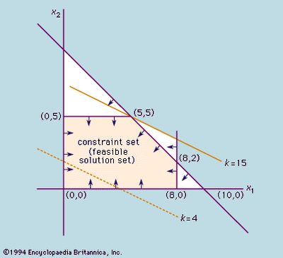
When plotted on a graph, these constraints form a polygonal region. This is the feasible solution set. Points outside this region violate one or more constraints.
To see how the simplex method identifies the optimal vertex, consider the objective function x1 + 2×2 = k. If you set k to 4, you get a line on the graph. As you increase k, you get parallel lines. The highest value of k that still touches the feasible region is the maximum possible profit.
In this example, the line for k = 15 touches the region at the point (5, 5). If k is higher, the line falls outside the feasible set. The optimal solution is producing equal quantities of each commodity.
Why Vertices Matter in Linear Programming
The result isn’t a coincidence. In linear problems, the optimal solution always occurs at a vertex. An extreme point.
This is a fundamental property of linear programming. The function is linear. The constraints are linear. The shape is a convex polygon (or polyhedron in higher dimensions). The peak of a linear function over a convex set is always at a corner.
You don’t need to check every point in the feasible region. You only need to check the vertices. The simplex method does exactly this. It hops from vertex to vertex. It climbs the surface of the feasible region. It stops when it can’t go higher.
Sometimes the optimum isn’t unique. An entire edge might yield the same maximum value. But the simplex method will still find one of those optimal points. It gives you a concrete answer. Actionable data.
For students and professionals alike, understanding this mechanic is key. It’s not just about solving equations. It’s about knowing how to navigate complex systems with limited resources. The simplex method provides the path.
The simplex method doesn’t just guess answers. It walks along the edges of a feasible region, checking vertices until it finds the best one. It starts by cleaning up the math. You take those messy linear inequalities and turn them into clean equalities. You do this by adding “slack variables.”
Think of slack as leftover capacity. If you have a constraint like $x_1 \le 8$, you add a variable $x_3$ such that $x_1 + x_3 = 8$. And remember, $x_3$ must be greater than or equal to zero. You do this for every constraint.
- $x_1 + x_3 = 8$ (with $x_3 \ge 0$)
- $x_2 + x_4 = 5$ (with $x_4 \ge 0$)
- $x_1 + x_2 + x_5 = 10$ (with $x_5 \ge 0$)
You also need a variable for the objective function itself. Let’s call it $x_0$. If your goal is to maximize $x_0 = x_1 + 2x_2$, you rewrite it as $x_1 + 2x_2 – x_0 = 0$.
Now the problem is simpler. Find non-negative values for $x_1$ through $x_5$. Make $x_0$ as large as possible.
Starting at the Origin
Where do you begin? The easiest spot is the origin. Set all the decision variables to zero. $x_1 = 0$. $x_2 = 0$.
This is a valid solution. It’s an extreme point. In fact, it’s the starting corner. The objective value $x_0$ is also zero. Not great, but it’s a legal move.
Can we do better? Yes. If you increase one of the variables from zero while keeping the other at zero, $x_0$ goes up. The question is which variable gives you the biggest bang for your buck.
Look at the objective equation: $x_1 + 2x_2 – x_0 = 0$. Rearranging for $x_0$, you get $x_0 = x_1 + 2x_2$.
Increasing $x_1$ adds 1 to the total. Increasing $x_2$ adds 2. $x_2$ is the clear winner. It produces the largest increase in $x_0$ per unit change. So, you pick $x_2$ and push it up.
Hitting the First Constraint
You can’t increase $x_2$ forever. The variables must stay non-negative. If you push $x_2$ past 5, something breaks. Specifically, look at the second constraint: $x_2 + x_4 = 5$.
If $x_2 = 6$, then $x_4$ becomes -1. That’s not allowed. The nonnegativity requirement acts as a hard stop. The limit is 5.
So you set $x_2 = 5$. What does the solution look like now?
- $x_2 = 5$
- $x_1 = 0$ (still zero)
- $x_4 = 0$ (this variable hit the limit, so it’s now zero)
- $x_3 = 8$ (since $0 + 8 = 8$)
- $